Defining functions
Functions are used for the definition of the functional form of
several potential types, e.g., embedded atom method (EAM)
potentials. atomicrex provides several
predefined functions as well as a mechanism to defined (almost)
arbitrary functional forms. Please consult the respective potential
sections for information regarding the positioning of a function block
in the potential block. All function elements have an id attribute
that is used to identify the respective function, e.g., for assigning
functions to different interaction types for EAM potentials via the <mapping> block.
Screening functions
Several pre-defined functions are intended to serve as “screening” (or cutoff) functions. They are constructed to satisfy the conditions \(f(0) = 1\) and \(f(r_c) = 0\) with (usually) smooth derivatives at the boundaries 1. These functions are (the normalization factor that enforces \(f(0) = 1\) has been omitted for clarity):
<exp-A>: This element sets up a type of exponential screening function,\[f(r; r_c) = \exp\left[ 1 / \left(r-r_c\right) \right],\]that is declared as follows:
<exp-A>
  <cutoff> 5.5 </cutoff>
</exp-A>
Here,
<cutoff>= \(r_c\).
<exp-B>: This element sets up another type of exponential screening function,\[f(r; r_c; n; \alpha; r_c^{(i)}) = \exp\left[ -\text{sign}(n) \cdot \alpha \big/ \left(1-x^n\right) \right]\]where \(x=\left(r - r_c^{(i)}\right) \big/ \left( r_c - r_c^{(i)} \right)\). This screening function is declared as follows:
<exp-B>
  <cutoff>    5.5 </cutoff>
  <rc>        2.8 </rc>
  <alpha>     1.0 </alpha>
  <exponent> -3.0 </exponent>
</exp-B>
Here,
<cutoff>= \(r_c\),<rc>= \(r_c^{(i)}\) (the inner cutoff radius, see figure below),<alpha>= \(\alpha\), and<exponent>= \(n\).
<exp-gaussian>: This element sets up a Gaussian distribution function multiplied with an exponential cutoff function\[f(r; r_c, n, \alpha, \sigma) = \exp\left[ -\text{sign}(n) \cdot \alpha \big/ \left(1-\left(r/r_c\right)^n\right) \right] \cdot \exp\left[ - r^2\big/2\sigma^2 \right] \big / \sigma\sqrt{2\pi}.\]The function is declared as follows:
<exp-gaussian>
  <cutoff>    5.5 </cutoff>
  <stddev>    2.8 </stddev>
  <alpha>     1.0 </alpha>
  <exponent> -3.0 </exponent>
</exp-gaussian>
Here,
<cutoff>= \(r_c\),<stddev>= \(\sigma\),<alpha>= \(\alpha\), and<exponent>= \(n\).
The following figure illustrates the different screening functions using exemplary parameters.
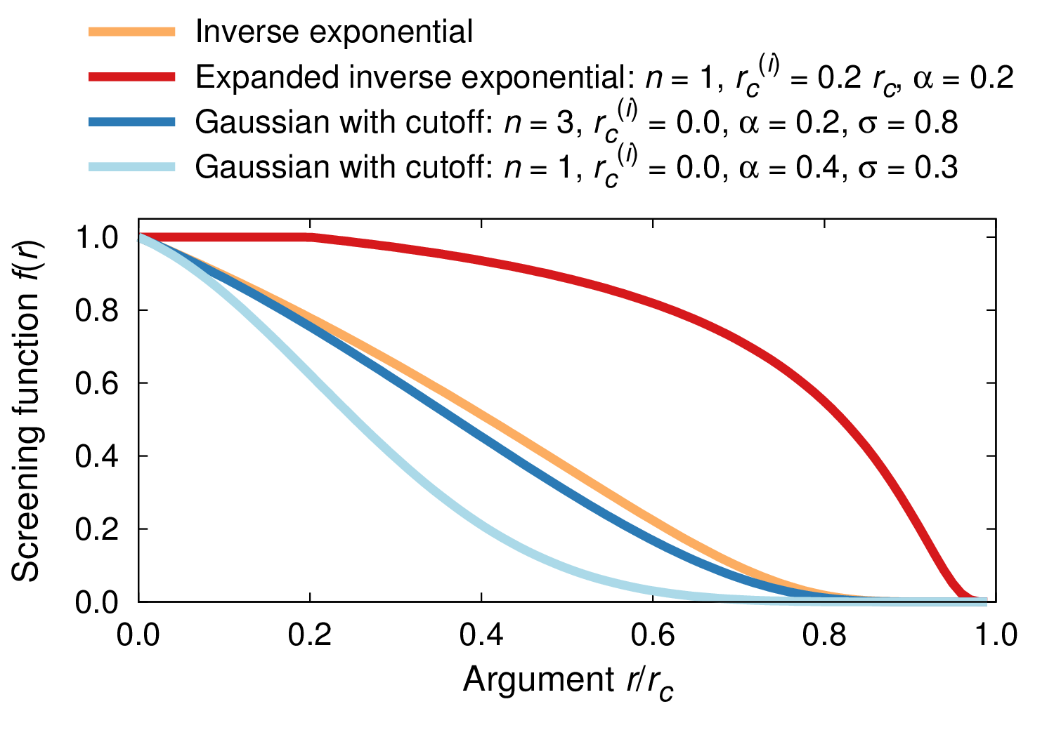
Screening functions using exemplary parameters.
Interpolation functions
Another set of functions is intended as interpolation functions and includes:
<poly>: A simple polynomial function defined as\[g(x) = \sum_{n=0}^P a_n x^n\]with the boundary conditions \(f(0) = 1\) and \(f(r_c) = 0\), where \(r_c\) is the upper cutoff, can be set up as follows:
<poly>
  <cutoff>5.5</cutoff>
  <coefficients>
    <coeff n="1" value="2.3" enabled="True" reset="False" min="1.0" max="7.0">
    <coeff n="2" value="1.1" enabled="True" reset="False" min="0.0" max="4.0">
    <coeff n="3" value="0.6" enabled="True" reset="False" min="0.0" max="4.0">
  </coefficients>
</poly>
Here,
<cutoff>defines the cutoff. The<coefficients>block specifies the coefficients. The value of \(a_n\) is set via thevalueattribute while thenattribute specifies \(n\). The attributesenabled,reset,min, andmaximplement the usual DOF features described here. The zero-th order coefficient \(a_0\) cannot be set by the user as it is fixed by the boundary conditions.
<spline>: A natural cubic spline function can be declared as follows:<spline> <cutoff>5.5</cutoff> <nodes> <node x="0" y="10" enabled="true" /> <node x="0.2" y="-0.3" enabled="true" /> <node x="0.5" y=" 0.1" enabled="true" /> <node x="0.7" y="-0.1" enabled="true" /> <node x="0.85" y=" 0.4" enabled="true" /> <node x="5.5" y=" 0" enabled="true" /> </nodes> </spline>
Here,
<cutoff>defines the cutoff. The<nodes>block specifies the nodal points of the spline. Each node is associated with a pair \((x,y)\) provided by the attributesxandy. The attributesenabled,reset,min, andmaximplement the usual DOF features described here. Note that only the \(y\) value is varied during optimization while the \(x\) value is kept fixed.It is possible to specify the first derivatives at the end points by using the optional parameter attributes
derivative-leftandderivative-rightas follows:<spline> <derivative-left> 123.0 </derivative-left> <derivative-right> -456.0 </derivative-right> ... </spline>
If these attributes are left unspecified they default to zero. An example for the use of splines can be found here.
<constant>: A constant “function” can be set up using:<constant> 2.1 </constant>
Specialized functions
atomicrex includes a few functions that are immediately suitable for instance as functional forms for pair potentials.
<morse-A>: The original Morse potential (typeA) is defined as\[V(r) = D_0 \left[ \exp\left(-2 \alpha (r-r_0) \right) - 2 \exp\left(-\alpha (r-r0) \right) \right]\]where the parameters \(D_0\) and \(r_0\) determine the cohesive energy and the optimum bond length, respectively, while the parameter \(\alpha\) affects the curvature of the potential curve and thus the stiffness. Note that the Morse potential has no “built-in” cutoff whence it must be combined with a screening (cutoff) function. The following block illustrates the specification of a standard Morse potential in the input file. It also provides an example for how to specify the fit parameters (
<fit-dof>blocks) and the insertion of a screening function via a<screening>block:<morse-A> <D0> 0.3 </D0> <r0> 3.0 </r0> <beta> 1.8 </beta> <fit-dof> <D0 enabled="true" /> <r0 enabled="true" /> <beta enabled="false" /> </fit-dof> <screening> <exp-B> <cutoff> 5.5 </cutoff> <rc> 0.0 </rc> <alpha> 1.0 </alpha> <exponent> -3.0 </exponent> <fit-dof> <alpha enabled="false" /> <exponent enabled="false" /> </fit-dof> </exp-B> </screening> </morse-A>
<morse-B>: A generalized Morse potential (variantB) as used for example in analytic bond-order potentials but also in some embedded atom method (EAM) potentials [MisMehPap01] is available as well. It is defined as\[V(r) = \underbrace{\frac{D_0}{S-1} \exp\left(- \beta \sqrt{2 S} (r-r_0) \right)}_{V_R} - \underbrace{\frac{D_0 S}{S-1} \exp\left(- \beta \sqrt{2/S} (r-r_0) \right)}_{V_A} + \delta.\]As in the original Morse potential, the parameters \(D_0\) and \(r_0\) determine the cohesive energy and the optimum bond length, respectively. The parameter \(\beta\) affects the curvature of the potential curve and thus the stiffness. The \(S\) parameter modifies the anharmonicity and can be set via the slope of the Pauling relation [AlbNorAve02], [AlbNorNor02], [ErhAlb05]. The entire potential can be shifted using the \(\delta\) parameter. With \(S=2\) and \(\delta=0\), one recovers the original Morse potential.
The following block illustrates the specification of a modified Morse
potential (variant B) in the input file:
<morse-B>
  <D0>   0.3 </D0>
  <r0>   3.0 </r0>
  <beta> 1.8 </beta>
  <S>    2.1 </S>
</morse-B>
<morse-C>: A generalized Morse potential (variantC) in the style used in the Tersoff potential is available as well. It is defined as\[\underbrace{A \exp\left(- \lambda r \right)}_{V_R} - \underbrace{B \exp\left(- \mu r \right)}_{V_A} + \delta.\]Note that the
<morse-B>form is usual preferred since the parameters have an immediate physical interpretation. Also the parameters \(A\) and \(B\) in the<morse-C>form can vary over a very large range, occasionally causing numerical instabilities that can strongly interfere with the fitting process. The format of a<morse-C>block is equivalent to the definition of<morse-A>and<morse-B>functions.
<gaussian>: The Gaussian function is defined as\[V(r) = a \exp\left(-\eta (r-\mu)^2 \right)\]with the three parameters \(a\) (the prefactor), \(\eta\) and \(\mu\). Note that the Gaussian function has no “built-in” cutoff, but -as for any function- you can still specify a hard cutoff the optional
cutoffattribute or apply a screening function using the<screening>element. The following block exemplifies the specification of a Gaussian function in the input file. block:<gaussian> <prefactor> 1.0 </prefactor> <eta> 3.0 </eta> <mu> 1.8 </mu> <fit-dof> <prefactor enabled="true" /> <eta enabled="false" /> <mu enabled="true" /> </fit-dof> </gaussian>
Combination functions
atomicrex provides furthermore two convenience functions,
<sum> and <product>, which allow one to combine two or more
function blocks without the need to explicitly integrate them into
one. For example, one could add two screening type functions using the
following set up:
<sum>
  <exp-A>
    <cutoff> 5.5 </cutoff>
  </exp-A>

  <exp-B>
    <cutoff>    5.5 </cutoff>
    <rc>        2.8 </rc>
    <alpha>     1.0 </alpha>
    <exponent> -3.0 </exponent>
  </exp-B>
</sum>
The <sum> operation is used in the example that demonstrates the
construction of an EAM potential with user defined functions to combine two pair
potentials.
User defined functions
atomicrex links to the muparser math parser library, which
provides enormous flexibility for defining functional forms. The
following input file block illustrates the definition of actually two
such user-defined function (one for the pair potential V and one for
the screening function rho_screening):
<user-function id="V">
  <input-var> r </input-var>
  <expression> A*exp(-lambda*r) </expression>
  <derivative> -lambda*A*exp(-lambda*r) </derivative>
  <param name="A"> 500 </param>
  <param name="lambda"> 2.73 </param>
  <fit-dof>
    <A/>
    <lambda/>
  </fit-dof>

  <screening>
    <user-function id="rho_screening">
      <cutoff>6.5</cutoff>
      <input-var>r</input-var>
      <expression> 1 - 1/(1 + ((r - cutoff) / h)^4) </expression>
      <derivative>
        4 * h^4 * (r-cutoff)^3 / ((h^4 + (r-cutoff)^4)^2)
      </derivative>
      <param name="h">3</param>
    </user-function>
  </screening>
</user-function>
Here, the following elements are used:
<input-var>: The identifier for the input variable used in the function definition.<expression>: The actual function, where the identifier specified in<input-var>is used as the argument of the function.<derivative>: The analytic derivative of the function specified in<expression>.<param>: Introduce a parameter that appears in the function definition. The name of the parameter is specified using thenameattribute. Typically there are several parameters.<fit-dof>: This element is used to declare the parameters that are to be adjusted during the optimization process. The parameters are provided as a list of subelements of the<fit-dof>block, where the name of the element is simply the name provided via thenameattribute in the<param>element.<screening>: The screening block allows one to integrate a screening (or cutoff) function, which provides a container for a function object.
A complete input file can be found in the example that demonstates the construction of an EAM potential with user defined functions.
Footnotes
- 1
Some potentials such as Tersoff and analytic bond-order potentials have built-in cutoff functions that are handled directly by the potential routine.